Neural Model
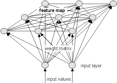
Let’s look at a highly simplified arrangement of the sensory input being received by a layer of neurons. In the Kohonen model of neural connections (Figure 10.1) each neuron in the input layer is connected (has a synapse) to each neuron in the receiving layer. Also, each neuron in the receiving layer is connected to every other neuron in the receiving layer. In combination with Hebb’s law and neurotransmitters (inhibitory as well as excitatory), this arrangement leads to selection of a neuron in the receiving layer with activity depression of distant neurons in the receiving layer.
Let’s start with a very small number of sensory neurons (35) being processed by 100 receiving neurons. Compare this with the optical nerve’s one million input signals being handled by many millions of receiving neurons in the cortex’s occipital lobe.
The sample network (Figure 10.2) has 35 sensory neurons ready to receive input. The result of the inputs they receive is delivered to the layer of 100 receiving neurons. At the same time, the triggered sensory neurons send a signal to each receiving neuron synaptic gap. In the receiving layer each of the 100 neurons notifies the other receiving neurons that it has received a signal. The efficiency of the synaptic transmissions (how much of the electrical potential crosses the gap) is affected by each transmission across it. That is an expression of [tooltip tip=”When an axon of cell A is near enough to excite cell B and repeatedly or persistently takes part in firing it, some growth process or metabolic change takes place in one or both cells such that A’s efficiency, as one of the cells firing B, is increased.” placement=”right”]Hebb’s law[/tooltip].
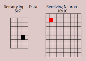
One neuron in the sensory layer has been stimulated, for example a photon has struck a retina cell. After repeated occurrences of this sensory cell being triggered, the sensory layer will settle on a cell, marked red, in the receiving layer.
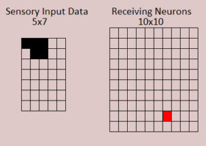
In Figure 10.3, a pattern of neurons are routinely stimulated by sensory experience. That set of neurons develops a set of synaptic weightings that trigger one of the receiving layer’s neurons.
Of course, more insight into how this assigning and learning takes place is needed. Let’s start with cortical interconnections.
Interconnections
Is the cortex arranged in the pattern that the Kohonen model postulates?
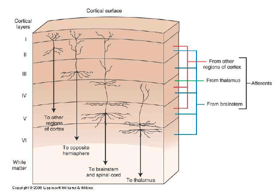
Certainly not exactly. Even in Figure 10.4 which is much simplified, more complexity exists that in the Kohonen model. However, enough strong similarities exist to use it as a working hypothesis, to see where it leads. The cortex has a quite uniform structure (Figure 10.4), comprising of six levels of neurons with a routine pattern of layer usage.
Training or Learning
At the very creation of the connections, synaptic efficiencies between the sensory and the receiving layers are random. It is only by repeated experience that specific inputs become linked to a winning neuron, by adjusted connectivity efficiencies at the synapse. From our conception, early in the womb, we are bombarded with a variety of inputs from our senses. Initially, there is a randomness to which receiving neuron fires in response to an input; however, [tooltip tip=”states the connection between two neurons increase if both of them are active at the same time” placement=”right”] according to Hebb’s Learning Law, [/tooltip]neurons that fire together are more likely to fire together again. The repeated, coordinated firing of neurons slowly shifts the efficiencies of the synaptic connections from the sensory layer to the receiving layer, so that eventually one neuron in the receiving layer routinely fires for each particular input that is received. The interconnections within the receiving layer are critical to this homing in on a final neuron. This is accomplished because they inhibit distant neurons and only excite immediate neighboring cells. The identification between the input data and an internal neuron has been learned.
Learning is completed when all normal inputs are associated with particular winning neurons and all the interconnections are steady. Once the learning mode is supplanted by use, the winning neuron activation is communicated to other areas of the brain for further processing. The learned category is available. There are two main physiological correlates that affect whether we are in heightened learning mode or in routine use of learned categories. The first is the [tooltip tip=”Gamma Amino Butyric Acid. The brain’s main inhibitory transmitter” placement=”right”]GABA[/tooltip] level, which affects the ease with which synaptic efficiency changes with new input. The second is the myelination status of the output axon. When a neuron’s axon has been sheathed with myelin, its output is rapidly sent to other areas of the brain for subsequent use.
Many Layers
The same layout of input layer and receiving layer occurs in many steps from initial sense data all the way up to the consideration of actions that all your sense data, knowledge, and goals prompt you to consider. Input discordant with the learned categories will be assigned to an existing category (winning neuron) with coincident adjustment of synaptic weightings. If the input is vastly different from any input learned during the training stage, it will be a shock to the system. In this case, no output may be created and anomalies like double outputs are possible. This situation is unlikely at the initial sensory layer. It is more likely downstream where the categories are not so fundamental.
Semantic Maps further develops implications.